[1]:

# To run this in Google Colab, uncomment the following line
# !pip install geometric_kernels

# If you want to use a version of the library from a specific branch on GitHub,
# say, from the "devel" branch, uncomment the line below instead
# !pip install "git+https://github.com/geometric-kernels/GeometricKernels@devel"

Matérn and Heat Kernels on Tori¶

This notebook shows how define and evaluate kernels on the two-dimensional torus $\mathbb{T}^2$.

Any torus $\mathbb{T}^d$ is a product manifold $\mathbb{T}^d = \mathbb{T}^1 \times \ldots \times \mathbb{T}^1$ where $\mathbb{T}^1 = \mathbb{S}_1$ is the circle. So this notebook also shows the basics of working with product manifolds.

Note: the kind of torus we consider here (product of circles) is the flat torus. Its Riemannian geometry is different from the Riemannian geometry that the often-visualized donut shape inherits from the ambient $\mathbb{R}^3$. Rather than that, its Riemannian geometry is the geometry of the product manifold while the geometry of each individual circle is inherited from the ambient $\mathbb{R}^2$ space. It follows that $\mathbb{T}^d$ can be embedded in $\mathbb{R}^{2 d}$ and the Riemannian geometry that this embedding inherits from the ambient $\mathbb{R}^{2 d}$ coincides with the Riemannian geometry of the flat torus. It is useful to think of the flat torus as the square ($d$-dimensional hypercube) with opposite sides glued together. Another way to think about the flat torus is that functions on the flat torus are exactly $2 \pi$-periodic functions (in each of the variables) on $\mathbb{R}^d$.

We use the numpy backend here.

Basics¶

[2]:

# Import a backend, we use numpy in this example.
import numpy as np
# Import the geometric_kernels backend.
import geometric_kernels

# Note: if you are using a backend other than numpy,
# you _must_ uncomment one of the following lines
# import geometric_kernels.tensorflow
# import geometric_kernels.torch
# import geometric_kernels.jax

# Import the spaces and an appropriate kernel.
from geometric_kernels.spaces import Circle, ProductDiscreteSpectrumSpace
from geometric_kernels.kernels import MaternGeometricKernel

import matplotlib as mpl
import matplotlib.pyplot as plt

INFO (geometric_kernels): Numpy backend is enabled. To enable other backends, don't forget to `import geometric_kernels.*backend name*`.
INFO (geometric_kernels): We may be suppressing some logging of external libraries. To override the logging policy, call `logging.basicConfig`.

Defining a Space¶

First we create a GeometricKernels space that corresponds to the 2-dimensional torus $\mathbb{T}^2$. We use ProductDiscreteSpectrumSpace which takes a number of DiscreteSpectrumSpace instances (e.g. Circle()) and constructs their product space.

ProductDiscreteSpectrumSpace has an optional parameter num_levels which determines the maximal order of approximation of the kernel (number of levels). ProductDiscreteSpectrumSpace uses the parameter num_levels for precomputation. There is a sensible default value for this parameter, so change it only if you know what you are doing.

[3]:

torus = ProductDiscreteSpectrumSpace(Circle(), Circle())

Defining a Kernel¶

First, we create a generic Matérn kernel.

To initialize MaternGeometricKernel you just need to provide a Space object, in our case this is the torus we have just created above.

There is also an optional second parameter num which determines the order of approximation of the kernel (number of levels). There is a sensible default value for each of the spaces in the library, so change it only if you know what you are doing.

A brief account on theory behind the kernels on product spaces can be found on this documentation page.

[4]:

kernel = MaternGeometricKernel(torus)

To support JAX, our classes do not keep variables you might want to differentiate over in their state. Instead, some methods take a params dictionary as input, returning its modified version.

The next line initializes the dictionary of kernel parameters params with some default values.

Note: our kernels do not provide the outputscale/variance parameter frequently used in Gaussian processes. However, it is usually trivial to add it by multiplying the kernel by an (optimizable) constant.

[5]:

params = kernel.init_params()
print('params:', params)

params: {'nu': array([inf]), 'lengthscale': array([1.])}

To define two different kernels, Matern-3/2 and Matern-∞ (aka heat, RBF, squared exponential, diffusion), we need two different versions of params:

[6]:

LENGTHSCALE = 0.5

params["lengthscale"] = np.array([LENGTHSCALE])
params_32  = params.copy()
params_inf = params.copy()
del params
params_32["nu"]  = np.array([3/2])
params_inf["nu"] = np.array([np.inf])

Now two kernels are defined and we proceed to evaluating both on a set of random inputs.

Evaluating Kernels on Random Inputs¶

We start by sampling 10 (uniformly) random points on the torus $\mathbb{T}^2$

[7]:

key = np.random.RandomState(1234)

key, xs = torus.random(key, 10)

print(xs)

[[1.2033522  2.24823221]
 [3.90882469 3.14784521]
 [2.7503245  4.29432427]
 [4.93455351 4.4780389 ]
 [4.90073254 2.3263541 ]
 [1.71274985 3.52609963]
 [1.73707615 3.16096475]
 [5.03831148 0.08650972]
 [6.02016711 4.85581287]
 [5.50364706 5.54579816]]

Now we evaluate the two kernel matrices.

[8]:

kernel_mat_32  = kernel.K(params_32,  xs, xs)
kernel_mat_inf = kernel.K(params_inf, xs, xs)

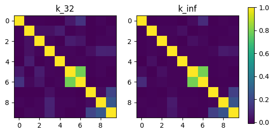
Finally, we visualize these matrices using imshow.

[9]:

# find common range of values
minmin = np.min([np.min(kernel_mat_32), np.min(kernel_mat_inf)])
maxmax = np.max([np.max(kernel_mat_32), np.max(kernel_mat_inf)])

fig, (ax1, ax2) = plt.subplots(nrows=1, ncols=2)
cmap = plt.get_cmap('viridis')

ax1.imshow(kernel_mat_32, vmin=minmin, vmax=maxmax, cmap=cmap)
ax1.set_title('k_32')

ax2.imshow(kernel_mat_inf, vmin=minmin, vmax=maxmax, cmap=cmap)
ax2.set_title('k_inf')

# add space for color bar
fig.subplots_adjust(right=0.85)
cbar_ax = fig.add_axes([0.88, 0.25, 0.02, 0.5])

# add colorbar
sm = plt.cm.ScalarMappable(cmap=cmap,
                           norm=plt.Normalize(vmin=minmin, vmax=maxmax))
fig.colorbar(sm, cax=cbar_ax)

plt.show()

Visualize Kernels¶

The torus $\mathbb{T}^2$ is one of the few manifolds we can easily visualize. Because of this, beyond kernel matrices, we will plot the functions $k_{\nu, \kappa}(\text{pole}, \cdot)$.

In practice, we visualize $k_{\nu, \kappa}($ base_point $, x)$ for $x \in `$ ``other_points`. We represent the torus as the square whose sides are assumed to be glued.

We define base_point and other_points in the next cell.

[10]:

base_point = np.array([[np.pi, 0.0]])

# define discretization
_NUM_PTS = 128

# generate a grid on the torus
x1s, x2s =  np.mgrid[0:2*np.pi:_NUM_PTS*1j, 0:2*np.pi:_NUM_PTS*1j]
other_points = np.c_[np.ravel(x1s), np.ravel(x2s)]

The next cell evaluates $k_{\nu, \kappa}($ base_point $, x)$ for $x \in `$ ``other_points` for $\nu$ either $3/2$ or $\infty$.

[11]:

kernel_vals_32  = kernel.K(params_32,  base_point, other_points)
kernel_vals_inf = kernel.K(params_inf, base_point, other_points)

Finally, we are ready to plot the results.

[12]:

fig, (ax1, ax2) = plt.subplots(figsize=(12.8, 4.8), nrows=1, ncols=2)

cmap = plt.get_cmap('viridis')

# find common range of values
minmin_vis = np.min([np.min(kernel_vals_32), np.min(kernel_vals_inf)])
maxmax_vis = np.max([np.max(kernel_vals_32), np.max(kernel_vals_inf)])

ax1.imshow( kernel_vals_32.reshape(_NUM_PTS, _NUM_PTS), vmin=minmin_vis, vmax=maxmax_vis, cmap=cmap)
ax2.imshow(kernel_vals_inf.reshape(_NUM_PTS, _NUM_PTS), vmin=minmin_vis, vmax=maxmax_vis, cmap=cmap)

# Remove axis
ax1.set_axis_off()
ax2.set_axis_off()

# plot the base point
ax1.scatter(x=[0, _NUM_PTS-1], y=[_NUM_PTS//2, _NUM_PTS//2], c='r', s=25)
ax2.scatter(x=[0, _NUM_PTS-1], y=[_NUM_PTS//2, _NUM_PTS//2], c='r', s=25)


ax1.set_title(r'$k_{3/2, \kappa}($base_point, other_points$)$')
ax2.set_title('$k_{\infty, \kappa}($base_point, other_points$)$')

# add color bar
sm = plt.cm.ScalarMappable(cmap=cmap,
                           norm=plt.Normalize(vmin=minmin_vis, vmax=maxmax_vis))
fig.subplots_adjust(right=0.85)
cbar_ax = fig.add_axes([0.88, 0.25, 0.02, 0.5])
fig.colorbar(sm, cax=cbar_ax)

plt.show()

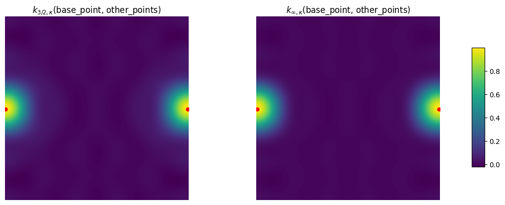
Notice how the kernel is getting “cut” on the left and continues on the right. This is because the sides of this rectangle are actually glued together.

Product Kernel vs Kernel on the Product Space¶

Here we describe an alternative way to define a kernel on torus, as a product kernel. The theory behind such kernels is briefly described on this documentation page.

Basically, a product kernel is a product of kernels. The advantage of using it is that it maintains a separate lengthscale for each of the factors of the product space, i.e. for each of the circles that make the torus. This allows you to use ARD, as in Rasmussen and Williams (2006). Also, we only support products of discrete spectrum spaces (via ProductDiscreteSpectrumSpace), whereas product kernels (ProductGeometricKernel) can be defined on arbitrary products of GeometricKernels spaces.

Note: product kernels do not coincide with kernels on product spaces unless $\nu = \infty$ and all lengthscales coincide. We will demonstrate this below.

We import the ProductGeometricKernel class

[13]:

from geometric_kernels.kernels import ProductGeometricKernel

We define a new generic product_kernel as the product of two MaternKarhunenLoeveKernel on the Circle, initialize and set its paramters.

[14]:

product_kernel = ProductGeometricKernel(MaternGeometricKernel(Circle(), 30),
                                        MaternGeometricKernel(Circle(), 30))
product_params = product_kernel.init_params()
print('params:', product_params)

product_params["lengthscale"] = np.array([LENGTHSCALE, LENGTHSCALE])
product_params_32  = product_params.copy()
product_params_inf = product_params.copy()
del product_params
product_params_32["nu"]  = np.array([3/2, 3/2])
product_params_inf["nu"] = np.array([np.inf, np.inf])

params: {'nu': array([inf, inf]), 'lengthscale': array([1., 1.])}

Next we compute the value of the product_kernel for $\nu = 3/2$ and for $\nu = \infty$. After this we compute the difference between the values of the product_kernel and the kernel.

[15]:

product_kernel_vals_32  = product_kernel.K(product_params_32,  base_point, other_points)
product_kernel_vals_inf = product_kernel.K(product_params_inf, base_point, other_points)
product_diff_32  = np.abs(kernel_vals_32  - product_kernel_vals_32)
product_diff_inf = np.abs(kernel_vals_inf - product_kernel_vals_inf)

We visualize the kernel and product_kernel for $\nu = 3/2$ as well as the difference between them.

[16]:

fig, (ax1, ax2, ax3) = plt.subplots(figsize=(12.8, 4.8), nrows=1, ncols=3)

cmap = plt.get_cmap('viridis')

# find common range of values
product_minmin_vis_32 = np.min([np.min(kernel_vals_32), np.min(product_kernel_vals_32)])
product_maxmax_vis_32 = np.max([np.max(kernel_vals_32), np.max(product_kernel_vals_32)])

ax1.imshow(        kernel_vals_32.reshape(_NUM_PTS, _NUM_PTS), vmin=product_minmin_vis_32, vmax=product_maxmax_vis_32, cmap=cmap)
ax2.imshow(product_kernel_vals_32.reshape(_NUM_PTS, _NUM_PTS), vmin=product_minmin_vis_32, vmax=product_maxmax_vis_32, cmap=cmap)
ax3.imshow(       product_diff_32.reshape(_NUM_PTS, _NUM_PTS), vmin=product_minmin_vis_32, vmax=product_maxmax_vis_32, cmap=cmap)


# Remove axis
ax1.set_axis_off()
ax2.set_axis_off()
ax3.set_axis_off()

# plot the base point
ax1.scatter(x=[0, _NUM_PTS-1], y=[_NUM_PTS//2, _NUM_PTS//2], c='r', s=25)
ax2.scatter(x=[0, _NUM_PTS-1], y=[_NUM_PTS//2, _NUM_PTS//2], c='r', s=25)
ax3.scatter(x=[0, _NUM_PTS-1], y=[_NUM_PTS//2, _NUM_PTS//2], c='r', s=25)

ax1.set_title(r'$k_{3/2, \kappa}^{T^2}($base_point, other_points$)$')
ax2.set_title('$k_{3/2, \kappa}^{S_1} \otimes k_{3/2, \kappa}^{S_1}($base_point, other_points$)$')
ax3.set_title('Difference')

# add color bar
sm = plt.cm.ScalarMappable(cmap=cmap,
                           norm=plt.Normalize(vmin=product_minmin_vis_32, vmax=product_maxmax_vis_32))
fig.subplots_adjust(right=0.85)
cbar_ax = fig.add_axes([0.88, 0.25, 0.02, 0.5])
fig.colorbar(sm, cax=cbar_ax)

plt.show()

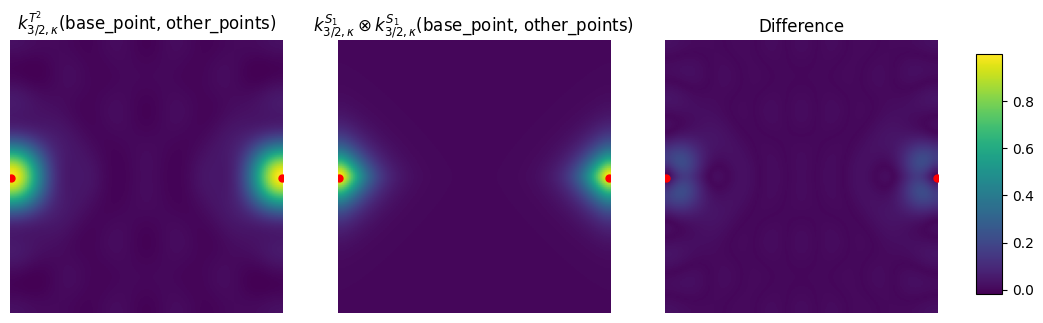
We see that the kernel differs from the product_kernel, despite having the same parameters.

We visualize the kernel and product_kernel for $\nu = \infty$ as well as the difference between them.

[17]:

fig, (ax1, ax2, ax3) = plt.subplots(figsize=(12.8, 4.8), nrows=1, ncols=3)

cmap = plt.get_cmap('viridis')

# find common range of values
product_minmin_vis_inf = np.min([np.min(kernel_vals_inf), np.min(product_kernel_vals_inf)])
product_maxmax_vis_inf = np.max([np.max(kernel_vals_inf), np.max(product_kernel_vals_inf)])

ax1.imshow(        kernel_vals_inf.reshape(_NUM_PTS, _NUM_PTS), vmin=product_minmin_vis_inf, vmax=product_maxmax_vis_inf, cmap=cmap)
ax2.imshow(product_kernel_vals_inf.reshape(_NUM_PTS, _NUM_PTS), vmin=product_minmin_vis_inf, vmax=product_maxmax_vis_inf, cmap=cmap)
ax3.imshow(       product_diff_inf.reshape(_NUM_PTS, _NUM_PTS), vmin=product_minmin_vis_inf, vmax=product_maxmax_vis_inf, cmap=cmap)


# Remove axis
ax1.set_axis_off()
ax2.set_axis_off()
ax3.set_axis_off()

# plot the base point
ax1.scatter(x=[0, _NUM_PTS-1], y=[_NUM_PTS//2, _NUM_PTS//2], c='r', s=25)
ax2.scatter(x=[0, _NUM_PTS-1], y=[_NUM_PTS//2, _NUM_PTS//2], c='r', s=25)
ax3.scatter(x=[0, _NUM_PTS-1], y=[_NUM_PTS//2, _NUM_PTS//2], c='r', s=25)

ax1.set_title(r'$k_{\infty, \kappa}^{T^2}($base_point, other_points$)$')
ax2.set_title('$k_{\infty, \kappa}^{S_1} \otimes k_{\infty, \kappa}^{S_1}($base_point, other_points$)$')
ax3.set_title('Difference')

# add color bar
sm = plt.cm.ScalarMappable(cmap=cmap,
                           norm=plt.Normalize(vmin=product_minmin_vis_inf, vmax=product_maxmax_vis_inf))
fig.subplots_adjust(right=0.85)
cbar_ax = fig.add_axes([0.88, 0.25, 0.02, 0.5])
fig.colorbar(sm, cax=cbar_ax)

plt.show()

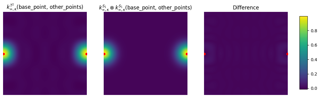
We see that the kernel and the product_kernel are the same in this case, as theory predicts.

Feature Maps and Sampling¶

Here we show how to get an approximate finite-dimensional feature map for heat and Matérn kernels on the torus, i.e. such $\phi$ that

\[k(x, x') \approx \langle \phi(x), \phi(x') \rangle_{\mathbb{R}^M}.\]

This might be useful for speeding up computations. We showcase this below by showing how to efficiently sample the Gaussian process $\mathrm{GP}(0, k)$.

For a brief theoretical introduction into feature maps, see this documentation page.

Defining a Feature Map¶

The simplest way to get an approximate finite-dimensional feature map is to use the default_feature_map function from geometric_kernels.kernels. It has an optional keyword argument num which determines the number of features, the $M$ above. Below we rely on the default value of num.

[18]:

from geometric_kernels.kernels import default_feature_map

feature_map = default_feature_map(kernel=kernel)

The resulting feature_map is a function that takes the array of inputs and parameters of the kernel. There is also an optional parameter normalize that determines if $\langle \phi(x), \phi(x) \rangle_{\mathbb{R}^M} \approx 1$ or not. For the (hyper)torus, normalize follows the standard behavior of MaternKarhunenLoeveKernel, being True by default.

feature_map outputs a tuple. Its second element is $\phi(x)$ evaluated at all inputs $x$. Its first element is either None for determinstic feature maps, or contains the updated key for randomized feature maps which take key as a keyword argument. For default_feature_map on a ProductDiscreteSpectrumSpace space, the first element is None since the feature map is deterministic.

In the next cell, we evaluate the feature map at random points, using params_32 as kernel parameters. We check the basic property of the feature map: $k(x, x') \approx \langle \phi(x), \phi(x') \rangle_{\mathbb{R}^M}$.

[19]:

# xs are random points from above
_, embedding = feature_map(xs, params_32)

print('xs (shape = %s):\n%s' % (xs.shape, xs))
print('')
print('emedding (shape = %s):\n%s' % (embedding.shape, embedding))

kernel_mat_32  = kernel.K(params_32,  xs, xs)
kernel_mat_32_alt = np.matmul(embedding, embedding.T)

print('')
print('||k(xs, xs) - phi(xs) * phi(xs)^T|| =', np.linalg.norm(kernel_mat_32 - kernel_mat_32_alt))

xs (shape = (10, 2)):
[[1.2033522  2.24823221]
 [3.90882469 3.14784521]
 [2.7503245  4.29432427]
 [4.93455351 4.4780389 ]
 [4.90073254 2.3263541 ]
 [1.71274985 3.52609963]
 [1.73707615 3.16096475]
 [5.03831148 0.08650972]
 [6.02016711 4.85581287]
 [5.50364706 5.54579816]]

emedding (shape = (10, 79)):
[[ 2.20941641e-01 -1.77201327e-01  2.20282049e-01  1.01558006e-01
   2.63837948e-01 -8.20588337e-02  1.02008762e-01 -2.13180970e-01
   2.65008968e-01 -4.67241284e-02 -2.13017530e-01 -1.61796025e-01
   1.46224685e-01 -2.20048929e-02 -1.00321356e-01 -5.71665986e-02
  -2.60625250e-01  1.32953172e-01 -1.65276398e-01 -1.20157684e-01
   1.49370104e-01  3.70909012e-02  1.69099188e-01 -3.35212520e-02
  -1.52824987e-01  1.38996113e-01  6.91272842e-02 -1.38512143e-01
  -7.00919906e-02  6.66250650e-02  3.31348101e-02  1.73085521e-01
   8.60810549e-02  1.15844560e-01 -1.44008385e-01  5.86214004e-02
  -7.28732814e-02 -1.17277704e-01 -5.83260139e-02  1.05990832e-01
   5.27126854e-02  3.37500180e-02  1.53867942e-01  1.70786900e-02
   7.78625623e-02 -9.84010909e-02  4.53492214e-02  1.09267048e-02
  -1.07795796e-01 -4.78452886e-02  2.20500257e-02 -1.24297465e-01
   5.72838494e-02 -9.27003297e-03  1.15237390e-02  9.14521446e-02
  -1.13685750e-01 -1.12300848e-01 -5.58508617e-02 -5.68281586e-02
  -2.82624902e-02  8.73722809e-02 -4.02664734e-02 -7.89635233e-02
   3.63912053e-02 -2.80179483e-03 -1.27735163e-02  2.76406941e-02
   1.26015243e-01  1.85929182e-02 -7.41799261e-02  8.76401535e-02
  -4.03899255e-02  4.43489841e-02 -2.04387155e-02  9.76578668e-03
   4.85684310e-03 -9.63429298e-02 -4.79144701e-02]
 [ 2.20941641e-01 -2.82703673e-01 -1.76764417e-03 -2.03503918e-01
  -1.96241297e-01  2.62330284e-01  1.64025671e-03  2.52968275e-01
   1.58171944e-03  2.18064613e-01  2.72706546e-03  7.92165549e-03
   2.17937743e-01 -2.05788857e-01 -2.57354770e-03 -1.98444691e-01
  -2.48170327e-03 -1.03851144e-02 -6.49343772e-05 -2.85711541e-01
  -1.78645128e-03  8.47538576e-03  1.05991208e-04  2.33171771e-01
   2.91599208e-03 -1.55209609e-01 -2.91171278e-03  1.03626831e-01
  -1.15585383e-01  1.49077536e-01  2.79667586e-03  1.43757276e-01
   2.69686845e-03 -1.38268895e-01 -8.64545560e-04  1.54225147e-01
   9.64314254e-04 -6.41179323e-03 -1.20284436e-04 -1.76398954e-01
  -3.30922224e-03  1.17842613e-01  1.47371238e-03 -1.31441669e-01
  -1.64377902e-03  1.08314288e-01  2.70953048e-03 -1.08062252e-01
   7.86614017e-03 -1.05531868e-01 -2.63992698e-03 -1.01765660e-01
  -2.54571361e-03  1.46261683e-01  9.14521583e-04 -1.06467788e-02
  -6.65704702e-05 -9.38173919e-02 -1.76000250e-03  1.04643934e-01
   1.96310706e-03  4.70877145e-03  1.17792029e-04  1.29546030e-01
   3.24065202e-03 -1.29319829e-01 -1.61724378e-03  9.41353599e-03
   1.17723497e-04 -7.64371895e-02 -2.39041865e-03  7.21727634e-02
   1.80543403e-03 -8.05015117e-02 -2.01378140e-03  1.07846980e-01
   2.02319582e-03 -7.85046995e-03 -1.47273831e-04]
 [ 2.20941641e-01 -1.14777842e-01 -2.58361256e-01 -2.61343785e-01
   1.07814274e-01  1.36777428e-01  3.07881622e-01 -5.64259032e-02
  -1.27012905e-01 -1.46188868e-01  1.61828388e-01  1.54647709e-01
  -1.53765075e-01  1.77170072e-01 -1.96124012e-01 -7.30894085e-02
   8.09086311e-02 -8.23124315e-02 -1.85282654e-01  8.18426425e-02
   1.84225174e-01 -1.10921599e-01  1.22788171e-01  1.10288527e-01
  -1.22087371e-01  1.47521453e-01  4.83313754e-02 -6.00217188e-02
   1.43163871e-01 -1.81965134e-01 -5.96159069e-02  7.50675541e-02
   2.45938341e-02  3.25152657e-02  7.31908243e-02 -7.75554485e-02
  -1.74574837e-01  1.18971688e-01  3.89778248e-02 -1.18292671e-01
  -3.87553632e-02  4.57580683e-02 -5.06533402e-02 -1.09142196e-01
   1.20818404e-01 -1.09744248e-02 -1.07790948e-01  6.20149651e-04
  -1.08346398e-01  1.37315336e-02  1.34871308e-01 -5.66478105e-03
  -5.56395557e-02 -3.40784362e-04 -7.67094712e-04  5.95384648e-02
   1.34019182e-01 -5.16483132e-02 -1.69211594e-02  1.23191615e-01
   4.03603686e-02 -9.31389143e-03 -9.14811670e-02  9.26073345e-03
   9.09590485e-02 -4.97527072e-04  5.50753319e-04  8.69229970e-02
  -9.62221592e-02 -6.63840461e-02  3.79673077e-02  4.23550857e-03
   4.16012222e-02 -1.01025398e-02 -9.92272822e-02  5.88256930e-04
   1.92726319e-04 -1.02774418e-01 -3.36712316e-02]
 [ 2.20941641e-01 -6.56481509e-02 -2.74981475e-01  6.22925615e-02
  -2.75760998e-01 -1.86467389e-02 -7.81058980e-02  8.25466672e-02
   3.45764565e-01 -1.94562913e-01  9.85133760e-02 -1.96905776e-01
  -9.37428815e-02 -5.62030821e-02  2.84574037e-02  2.48803672e-01
  -1.25977193e-01  5.99438781e-02  2.51087895e-01  2.85380754e-02
   1.19537900e-01  1.87964937e-01 -9.51726114e-02  8.94863280e-02
  -4.53097671e-02  1.00368062e-01  1.18426150e-01 -9.59727074e-02
   1.22015328e-01  2.95088681e-02  3.48180644e-02 -1.30631888e-01
  -1.54135004e-01  2.97365834e-02  1.24558110e-01 -3.78057374e-02
  -1.58357506e-01 -1.03062090e-01 -1.21604884e-01 -4.90657892e-02
  -5.78936408e-02  9.73761856e-02 -4.93046524e-02 -1.23799646e-01
   6.26836888e-02  6.41297054e-02 -8.73310222e-02  6.83085591e-02
   8.41027189e-02  1.91258407e-02 -2.60453281e-02 -8.46675878e-02
   1.15299251e-01 -2.14695391e-02 -8.99298068e-02 -2.64336803e-02
  -1.10723186e-01 -5.61869966e-02 -6.62960865e-02  7.14335878e-02
   8.42858241e-02 -6.92984644e-02  9.43697729e-02 -3.29916059e-02
   4.49275519e-02 -7.29358578e-02  3.69297389e-02 -8.97999318e-02
   4.54685547e-02 -7.04661127e-02 -2.97133807e-02 -3.95751310e-02
   5.38929131e-02  5.03140186e-02 -6.85169945e-02  4.40845112e-02
   5.20161380e-02  5.42776382e-02  6.40431989e-02]
 [ 2.20941641e-01 -1.93852221e-01  2.05780971e-01  5.29322096e-02
  -2.77709691e-01 -4.67880566e-02  4.96671727e-02  2.45474294e-01
  -2.60579622e-01 -1.30075579e-02 -2.17693398e-01 -2.02791600e-01
  -8.02195693e-02 -3.19285853e-03 -5.34354125e-02  1.67513837e-02
   2.80349754e-01  1.82299142e-01 -1.93516971e-01  7.21132370e-02
  -7.65507450e-02  1.29420794e-02  2.16597555e-01  5.11958105e-03
   8.56808792e-02  1.19143060e-01  9.95159889e-02 -8.31203226e-02
   1.31108782e-01  2.97652544e-02  2.48618654e-02 -1.56163887e-01
  -1.30438178e-01  7.60499311e-02 -8.07296848e-02 -1.19956390e-01
   1.27337940e-01 -1.25998004e-01 -1.05241681e-01 -4.98418357e-02
  -4.16311245e-02  5.63829690e-03  9.43620641e-02 -8.89349580e-03
  -1.48840800e-01 -1.07577261e-01  1.29019190e-02  7.90274999e-02
   7.41213925e-02 -2.72624953e-02  3.26963619e-03  1.43033121e-01
  -1.71541990e-02 -7.33456095e-02  7.78589520e-02 -6.87922397e-02
   7.30253892e-02 -5.77654958e-02 -4.82494779e-02  9.11156691e-02
   7.61056994e-02  1.19722659e-01 -1.43585367e-02  4.73594576e-02
  -5.67989813e-03 -5.64130944e-03 -9.44124817e-02 -5.29109122e-03
  -8.85512590e-02  4.54366044e-02 -6.15131939e-02  5.74967201e-02
  -6.89567682e-03 -9.06917192e-02  1.08768080e-02  6.05427805e-02
   5.05692456e-02  5.67842232e-02  4.74298555e-02]
 [ 2.20941641e-01 -2.62066757e-01 -1.06044831e-01 -3.99969227e-02
   2.79865571e-01  4.77950276e-02  1.93401699e-02 -3.34430295e-01
  -1.35326603e-01  1.56712773e-01  1.51659879e-01 -2.09351500e-01
  -6.10865110e-02 -2.90666418e-02 -2.81294453e-02  2.03384454e-01
   1.96826724e-01  2.54420379e-01  1.02950738e-01  7.42371241e-02
   3.00399156e-02 -1.60967723e-01 -1.55777637e-01 -4.69686465e-02
  -4.54542352e-02 -6.29130423e-02 -1.41917053e-01  6.41290924e-02
  -1.41371710e-01  1.18764895e-02  2.67905721e-02 -8.31019062e-02
  -1.87458390e-01 -7.93209402e-02 -3.20970724e-02  1.74861931e-01
   7.07575584e-02  6.86849705e-02  1.54937168e-01  2.00415340e-02
   4.52089955e-02  5.24088274e-02  5.07190082e-02 -1.15534545e-01
  -1.11809362e-01  3.54976289e-03  1.08290008e-01  9.13460198e-02
   5.82686128e-02 -6.79752828e-04 -2.07367199e-02  4.75635124e-03
   1.45098512e-01 -1.14611095e-01 -4.63771686e-02 -7.31091463e-02
  -2.95834815e-02 -2.35335972e-02 -5.30862702e-02  5.18794941e-02
   1.17027959e-01 -4.07832032e-03 -1.24414321e-01 -1.19000991e-03
  -3.63027576e-02  7.85597217e-02  7.60267185e-02  5.01123751e-02
   4.84966004e-02  2.63478134e-02 -7.17924144e-02  1.46375977e-03
   4.46538436e-02 -3.22683846e-03 -9.84387893e-02 -3.69526582e-02
  -8.33565212e-02 -2.35716908e-02 -5.31722003e-02]
 [ 2.20941641e-01 -2.82656154e-01 -5.47632805e-03 -4.67925094e-02
   2.78809886e-01  6.03085636e-02  1.16844963e-03 -3.59344347e-01
  -6.96212518e-03  2.17918002e-01  8.44728541e-03 -2.06132929e-01
  -7.11957013e-02 -4.72860818e-02 -1.83297857e-03  2.81750802e-01
   1.09216743e-02  2.70190269e-01  5.23480747e-03  9.33202946e-02
   1.80803616e-03 -2.20393515e-01 -8.54324519e-03 -7.61211270e-02
  -2.95072862e-03 -1.54974835e-01 -9.01671717e-03  7.42663886e-02
  -1.36319494e-01  3.42261733e-02  1.99134087e-03 -2.03934253e-01
  -1.18652649e-02 -9.90767097e-02 -1.91956395e-03  1.81860020e-01
   3.52345107e-03  1.66591758e-01  9.69261079e-03  5.75386819e-02
   3.34770493e-03  8.43976525e-02  3.27155651e-03 -1.54915911e-01
  -6.00509780e-03  1.08023050e-01  8.38732668e-03  8.52530208e-02
   6.68673987e-02 -2.42001396e-02 -1.87899227e-03  1.44194834e-01
   1.11958437e-02 -1.15370114e-01 -2.23524088e-03 -9.04894550e-02
  -1.75318999e-03 -6.71345411e-02 -3.90600943e-03  1.23228648e-01
   7.16966636e-03 -1.22199582e-01 -9.48804737e-03 -4.22061870e-02
  -3.27705132e-03  1.01955063e-01  3.95214487e-03  7.99674870e-02
   3.09982736e-03 -7.61160980e-02 -7.39578638e-03  5.15850802e-02
   4.00526480e-03 -9.46868717e-02 -7.35185430e-03 -8.49544885e-02
  -4.94280631e-03 -6.66332478e-02 -3.87684328e-03]
 [ 2.20941641e-01  2.81651971e-01  2.44265993e-02  9.05186404e-02
  -2.67826188e-01  1.16250551e-01  1.00819661e-02 -3.43961661e-01
  -2.98304807e-02  2.14825583e-01  3.75443914e-02 -1.73367480e-01
  -1.32300148e-01  9.01753640e-02  1.57596648e-02 -2.66810504e-01
  -4.66296326e-02 -2.26435396e-01 -1.96378767e-02 -1.72797322e-01
  -1.49860515e-02 -1.82730888e-01 -3.19353025e-02 -1.39445549e-01
  -2.43704601e-02  1.50038176e-01  3.98377532e-02 -1.28730487e-01
   8.67580689e-02  6.41003826e-02  1.70197698e-02 -1.89659954e-01
  -5.03580264e-02 -1.71125619e-01 -1.48410711e-02  1.15330320e-01
   1.00021580e-02 -1.35648303e-01 -3.60169909e-02 -1.03515899e-01
  -2.74852770e-02 -1.44215641e-01 -2.52041139e-02  9.71943071e-02
   1.69863434e-02  1.01925683e-01  3.67489005e-02  2.85975762e-02
   1.04506006e-01  4.41719683e-02  1.59260278e-02 -1.30695842e-01
  -4.71218670e-02  3.85626720e-02  3.34439320e-03  1.40922112e-01
   1.22216363e-02 -1.12661550e-01 -2.99136070e-02  7.59283894e-02
   2.01603120e-02 -9.69744174e-02 -3.49637413e-02 -7.40030930e-02
  -2.66815215e-02  3.37148425e-02  5.89223699e-03  1.23206369e-01
   2.15323896e-02  6.94312789e-02  3.20570669e-02 -8.43685164e-02
  -3.04187337e-02  5.68602647e-02  2.05007427e-02  2.75896614e-02
   7.32553640e-03  1.00822716e-01  2.67701900e-02]
 [ 2.20941641e-01  4.04083847e-02 -2.79806458e-01  2.72986733e-01
  -7.35032985e-02  5.02987549e-02 -3.48291983e-01 -1.35432384e-02
   9.37796841e-02 -2.09170956e-01 -6.17018934e-02  1.88597900e-01
  -1.09500887e-01 -2.64793186e-01 -7.81095105e-02  7.12971374e-02
   2.10314494e-02  3.53404624e-02 -2.44713806e-01 -2.05188498e-02
   1.42082063e-01 -1.93551510e-01 -5.70944211e-02  1.12376977e-01
   3.31493073e-02 -6.47520718e-02  1.41087455e-01  1.09366982e-01
  -1.10169706e-01 -8.34288073e-02  1.81781953e-01  2.24637016e-02
  -4.89458701e-02  2.08582823e-02 -1.44432452e-01 -2.10113765e-02
   1.45492548e-01 -6.36847539e-02  1.38761890e-01  3.69756876e-02
  -8.05658494e-02 -1.19297834e-01 -3.51908430e-02  1.20173448e-01
   3.54491343e-02  9.10017366e-02  5.88048510e-02  5.37159896e-02
  -9.40952657e-02  1.18936819e-01  7.68563568e-02 -3.20244447e-02
  -2.06940303e-02  1.03920247e-02 -7.19592144e-02 -1.82038967e-02
   1.26052251e-01 -4.13078347e-02  9.00051090e-02  4.16110231e-02
  -9.06657222e-02  9.41873212e-02  6.08633592e-02 -5.46856312e-02
  -3.53375717e-02 -6.16610439e-02 -1.81889648e-02  1.08012760e-01
   3.18619371e-02  5.02603291e-02 -5.76390263e-02  6.39957711e-02
   4.13537359e-02 -6.44654828e-02 -4.16572612e-02 -2.23651914e-02
   4.87312274e-02  3.91775083e-02 -8.53633681e-02]
 [ 2.20941641e-01  2.09269223e-01 -1.90081255e-01  2.01073583e-01
  -1.98730736e-01  1.91868899e-01 -1.74276373e-01 -1.89633302e-01
   1.72245758e-01  2.09084801e-02 -2.17077055e-01  2.55582235e-03
  -2.18066687e-01  1.94958136e-02 -2.02410399e-01 -1.92686545e-02
   2.00051976e-01  2.48027543e-03 -2.25285811e-03 -2.11620907e-01
   1.92217313e-01  2.62187183e-04 -2.72209272e-03 -2.23702130e-02
   2.32253130e-01 -9.28766704e-02 -1.24388202e-01 -1.07822503e-01
  -1.11681730e-01 -8.81419145e-02 -1.18047021e-01  8.71149123e-02
   1.16671574e-01 -1.06496564e-01  9.67318566e-02 -1.10308332e-01
   1.00194123e-01 -1.23789057e-03 -1.65788655e-03  1.05618724e-01
   1.41453426e-01 -1.17564669e-02  1.22058571e-01 -1.21772591e-02
   1.26427341e-01 -1.06356316e-01 -2.06799587e-02 -1.08318410e-01
  -2.53941261e-03 -1.02386666e-01 -1.99080986e-02  1.01193688e-01
   1.96761356e-02 -1.08525735e-01  9.85749730e-02 -2.54427314e-03
   2.31098785e-03  5.84128747e-02  7.82314057e-02  6.05036123e-02
   8.10314963e-02 -1.49176310e-03 -2.90058931e-04  1.27279518e-01
   2.47482733e-02 -1.24288416e-02  1.29039333e-01 -2.91381280e-04
   3.02519312e-03 -6.53818762e-02  3.96682279e-02  7.37374408e-02
   1.43375334e-02  7.63766816e-02  1.48507083e-02  6.46880833e-02
   8.66356897e-02  1.51654492e-03  2.03108376e-03]]

||k(xs, xs) - phi(xs) * phi(xs)^T|| = 2.5753823296802577e-15

Efficient Sampling using Feature Maps¶

GeometricKernels provides a simple tool to efficiently sample (without incurring cubic costs) the Gaussian process $f \sim \mathrm{GP}(0, k)$, based on an approximate finite-dimensional feature map $\phi$. The underlying machinery is briefly discussed in this documentation page.

The function sampler from geometric_kernels.sampling takes in a feature map and, optionally, the keyword argument s that specifies the number of samples to generate. It returns a function we name sample_paths.

sample_paths operates much like feature_map above: it takes in the points where to evaluate the samples and kernel parameters. Additionally, it takes in the keyword argument key that specifies randomness in the JAX style. sample_paths returns a tuple. Its first element is the updated key. Its second element is an array containing the value of samples evaluated at the input points.

[20]:

from geometric_kernels.sampling import sampler

sample_paths = sampler(feature_map, s=2)

# introduce random state for reproducibility (optional)
# `key` is jax's terminology
key = np.random.RandomState(seed=1234)

# new random state is returned along with the samples
key, samples = sample_paths(xs, params_32, key=key)

print('Two samples evaluated at the xs are:')
print(samples)

Two samples evaluated at the xs are:
[[ 0.31634816 -2.38559012]
 [-0.61819585  0.12209121]
 [ 0.8101087  -1.70702319]
 [-0.63509083  1.0057374 ]
 [ 0.1851223   0.51089693]
 [ 0.02621555  0.15314556]
 [-0.19946012  0.37070016]
 [ 0.25204997 -0.28420479]
 [-0.92386637  1.50608757]
 [ 2.0426702  -0.31522709]]

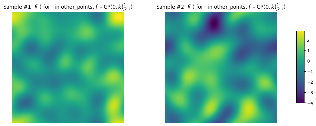
Visualizing Samples¶

Here we visualize samples as functions on the torus.

[21]:

key = np.random.RandomState(seed=1234)
key, samples = sample_paths(other_points, params_32, key=key)

sample1 = samples[:, 0]
sample2 = samples[:, 1]

fig, (ax1, ax2) = plt.subplots(figsize=(12.8, 4.8), nrows=1, ncols=2)

cmap = plt.get_cmap('viridis')

# find common range of values
minmin_vis = np.min([np.min(sample1), np.min(sample2)])
maxmax_vis = np.max([np.max(sample1), np.max(sample2)])

ax1.imshow(sample1.reshape(_NUM_PTS, _NUM_PTS), vmin=minmin_vis, vmax=maxmax_vis, cmap=cmap)
ax2.imshow(sample2.reshape(_NUM_PTS, _NUM_PTS), vmin=minmin_vis, vmax=maxmax_vis, cmap=cmap)

# Remove axis
ax1.set_axis_off()
ax2.set_axis_off()

ax1.set_title('Sample #1: $f(\cdot)$ for $\cdot$ in other_points, $f \sim \mathrm{GP}(0, k_{3/2, \kappa}^{T^2})$')
ax2.set_title('Sample #2: $f(\cdot)$ for $\cdot$ in other_points, $f \sim \mathrm{GP}(0, k_{3/2, \kappa}^{T^2})$')

# add color bar
sm = plt.cm.ScalarMappable(cmap=cmap,
                           norm=plt.Normalize(vmin=minmin_vis, vmax=maxmax_vis))
fig.subplots_adjust(right=0.85)
cbar_ax = fig.add_axes([0.88, 0.25, 0.02, 0.5])
fig.colorbar(sm, cax=cbar_ax)

plt.show()

Feature Maps and Sampling for Product Kernels¶

This functionality is not implemented yet, unfortunately.

Citation¶

If you are using (hyper)tori and GeometricKernels, please consider citing

@inproceedings{borovitskiy2020,
    title={Matérn Gaussian processes on Riemannian manifolds},
    author={Viacheslav Borovitskiy and Alexander Terenin and Peter Mostowsky and Marc Peter Deisenroth},
    booktitle={Advances in Neural Information Processing Systems},
    year={2020}
}

[ ]: