# To run this in Google Colab, uncomment the following line
# !pip install geometric_kernels

# If you want to use a version of the library from a specific branch on GitHub,
# say, from the "devel" branch, uncomment the line below instead
# !pip install "git+https://github.com/geometric-kernels/GeometricKernels@devel"

Gaussian Process Regression on a Mesh with GPJax

This notebooks shows how to fit a GPJax Gaussian process (GP) on a mesh.

This notebook is written for GPJax>=0.12.2 (Python-3.10) and GPJax<=0.13.2 (Python-3.11). GPJax is in active development and changes API frequently. We strive to support the most recent version of it, so the notebook will not work on the older versions.

# Import a backend, we use jax in this example.
import jax.numpy as jnp
import jax
import gpjax as gpx

# Import the geometric_kernels backend.
import geometric_kernels
import geometric_kernels.jax

# Import the Mesh space and the general-purpose MaternGeometricKernel
from geometric_kernels.spaces.mesh import Mesh
from geometric_kernels.kernels import MaternGeometricKernel

# The GPJax frontend of GeometricKernels
from geometric_kernels.frontends.gpjax import GPJaxGeometricKernel

# Sampling routines we will use to create a dummy dataset
from geometric_kernels.kernels import default_feature_map
from geometric_kernels.sampling import sampler
from geometric_kernels.utils.utils import make_deterministic

# Stuff
import numpy as np
import optax
import plotly.graph_objects as go
from plotly.subplots import make_subplots
from pathlib import Path

jax.config.update("jax_enable_x64", True)

import logging

for name in ("kaleido", "choreographer", "choreographer.browsers", "choreographer.utils"):
    logger = logging.getLogger(name)
    logger.setLevel(logging.WARNING)
    logger.propagate = False

INFO (geometric_kernels): Numpy backend is enabled. To enable other backends, don't forget to `import geometric_kernels.*backend name*`.
INFO (geometric_kernels): We may be suppressing some logging of external libraries. To override the logging policy, call `logging.basicConfig`.
/Users/vabor112/Downloads/GeometricKernels/.venv/lib/python3.11/site-packages/spherical_harmonics/fundamental_set.py:21: UserWarning: pkg_resources is deprecated as an API. See https://setuptools.pypa.io/en/latest/pkg_resources.html. The pkg_resources package is slated for removal as early as 2025-11-30. Refrain from using this package or pin to Setuptools<81.
  from pkg_resources import resource_filename
INFO (geometric_kernels): JAX backend enabled.

Mesh Plotting Utils for plotly

def update_figure(fig):
    """Utility to clean up figure"""
    fig.update_layout(scene_aspectmode="cube")
    fig.update_scenes(xaxis_visible=False, yaxis_visible=False, zaxis_visible=False)
    # fig.update_traces(showscale=False, hoverinfo="none")
    fig.update_layout(margin=dict(l=0, r=0, t=0, b=0))

    fig.update_layout(plot_bgcolor="rgba(0,0,0,0)", paper_bgcolor="rgba(0,0,0,0)")
    fig.update_layout(
        scene=dict(
            xaxis=dict(showbackground=False, showticklabels=False, visible=False),
            yaxis=dict(showbackground=False, showticklabels=False, visible=False),
            zaxis=dict(showbackground=False, showticklabels=False, visible=False),
        )
    )
    return fig

def plot_mesh(mesh: Mesh, vertices_colors = None, **kwargs):
    plot = go.Mesh3d(
        x=mesh.vertices[:, 0],
        y=mesh.vertices[:, 1],
        z=mesh.vertices[:, 2],
        i=mesh.faces[:, 0],
        j=mesh.faces[:, 1],
        k=mesh.faces[:, 2],
        intensity=vertices_colors,
        **kwargs
    )
    return plot

Defining a Space

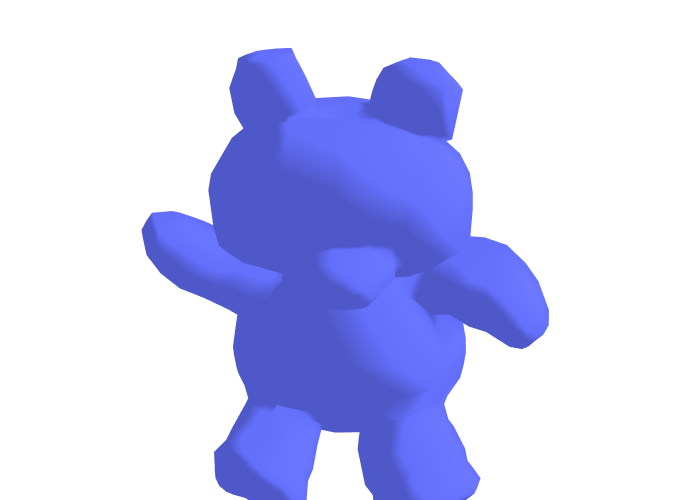
First, we create a GeometricKernels space that corresponds to a teddy bear mesh loaded from “../data/teddy.obj”

mesh = Mesh.load_mesh(str(Path.cwd().parent / "data" / "teddy.obj"))
print("Number of vertices in the mesh:", mesh.num_vertices)

Number of vertices in the mesh: 1598

Now we actually visualize the mesh.

# Define the camera
camera = dict(
    up=dict(x=0, y=1, z=0),
    center=dict(x=0, y=0, z=0),
    eye=dict(x=0, y=0.7, z=1.25)
)

plot = plot_mesh(mesh)
fig = go.Figure(plot)
update_figure(fig)
fig.update_layout(
    scene_camera=camera
)
fig.show("png")

Create a Dummy Dataset on the Mesh

We sample from the prior of a GP to create a simple dataset we can afterwards fit using an exact Gaussian process regression (GPR) model.

The input set \(X \in \mathbb{N}^{n \times 1}\) consists of indices enumerating vertices of the mesh. Consequently, the elements of \(X\) are in \([0, N_v-1]\), where \(N_v\) are the number of vertices in the mesh. We sample num_data of them into the tensor called xs_train. For test inputs xs_test, we use the whole \(X\).

num_data = 50
key = jax.random.PRNGKey(1234)

xs_train = jax.random.randint(key, minval=0, maxval=mesh.num_vertices, shape=(num_data, 1), dtype=jnp.int64)
xs_test = jnp.arange(mesh.num_vertices, dtype=jnp.int64)[:, None]
# print("xs_train:", xs_train)
# print("xs_test:", xs_test)

To generate the corresponding outputs ys_train and ys_test, we sample from the prior. To do this, we create a MaternGeometricKernel object and use the efficent sampling functionality of GeometricKernels.

base_kernel = MaternGeometricKernel(mesh)

params = base_kernel.init_params()
params["lengthscale"] = jnp.array([5.0], dtype=jnp.float64)
params["nu"]  = jnp.array([2.5], dtype=jnp.float64)

feature_map = default_feature_map(kernel=base_kernel)
sample_paths = make_deterministic(sampler(feature_map), key)

_, ys_train  = sample_paths(xs_train, params, normalize=True)
key, ys_test = sample_paths(xs_test,  params, normalize=True)

assert(jnp.allclose((ys_test[xs_train[:, 0]]), ys_train))

# print("ys_train:", ys_train)
# print((ys_test[xs_train])[:, :, 0])

Build a GPJax Model

Now we wrap the base_kernel created above into the GPJaxGeometricKernel to make an actual GPJax kernel.

Note: params are external to the base_kernel object, thus we need to pass them to the GPJaxGeometricKernel explicitly. Otherwise it will use params = base_kernel.init_params().

params = base_kernel.init_params()
params["lengthscale"] = jnp.array([3.0], dtype=jnp.float64)
params["nu"]  = jnp.array([2.5], dtype=jnp.float64)
kernel = GPJaxGeometricKernel(base_kernel=base_kernel,
                                        nu=params["nu"],
                                        lengthscale=params["lengthscale"],
                                        variance=1.0)

# Pass `trainable_nu=True` if you want optimizable nu.
# Note: if nu is initialized to jnp.inf, it will not be optimizable either way.

We use the data xs_train, ys_train and the GPJax kernel kernel to construct a GPJax model.

data = gpx.Dataset(X=xs_train, y=ys_train)

prior = gpx.gps.Prior(mean_function=gpx.mean_functions.Zero(), kernel=kernel)

likelihood = gpx.likelihoods.Gaussian(num_datapoints=num_data, obs_stddev=1e-4)

posterior = likelihood * prior

print("Initial model:")
print("kernel.nu =", prior.kernel.nu)
print("kernel.lengthscale =", prior.kernel.lengthscale)
print("kernel.variance =", prior.kernel.variance)
print("likelihood.obs_noise =", likelihood.obs_stddev)
print("")

mll = gpx.objectives.conjugate_mll
print("Initial negative log marginal likelihood:", -mll(posterior, data))

/Users/vabor112/Downloads/GeometricKernels/.venv/lib/python3.11/site-packages/gpjax/dataset.py:43: UserWarning:

X is not of type float64. Got X.dtype=int64. This may lead to numerical instability.

Initial model:
kernel.nu = [2.5]
kernel.lengthscale = PositiveReal( # 1 (8 B)
  value=Array([3.], dtype=float64),
  tag='positive'
)
kernel.variance = NonNegativeReal( # 1 (8 B)
  value=Array(1., dtype=float64, weak_type=True),
  tag='non_negative'
)
likelihood.obs_noise = NonNegativeReal( # 1 (8 B)
  value=Array(0.0001, dtype=float64, weak_type=True),
  tag='non_negative'
)

Initial negative log marginal likelihood: 46.515723209698976

Train the Model (Optimize Hyperparameters)

mll = jax.jit(mll, static_argnums=(0,))

print("Starting training...")
opt_posterior, history = gpx.fit(
    model=posterior,
    objective=lambda p, d: -mll(p, d),
    train_data=data,
    optim=optax.sgd(0.01),
    key=key,
    trainable=gpx.parameters.Parameter,
)
print("Final model:")
print("kernel.nu =", opt_posterior.prior.kernel.nu)
print("kernel.lengthscale =", opt_posterior.prior.kernel.lengthscale)
print("kernel.variance =", opt_posterior.prior.kernel.variance)
print("likelihood.obs_stddev =", opt_posterior.likelihood.obs_stddev)
print("")

print("Final negative log marginal likelihood:", -mll(opt_posterior, data))

Starting training...

/Users/vabor112/Downloads/GeometricKernels/.venv/lib/python3.11/site-packages/gpjax/dataset.py:43: UserWarning:

X is not of type float64. Got X.dtype=int64. This may lead to numerical instability.

Final model:
kernel.nu = [2.5]
kernel.lengthscale = PositiveReal( # 1 (8 B)
  value=Array([5.3273158], dtype=float64),
  tag='positive'
)
kernel.variance = NonNegativeReal( # 1 (8 B)
  value=Array(0.83287579, dtype=float64),
  tag='non_negative'
)
likelihood.obs_stddev = NonNegativeReal( # 1 (8 B)
  value=Array(9.90240582e-05, dtype=float64),
  tag='non_negative'
)

Final negative log marginal likelihood: 37.43092644541115

Draw Predictions and Evaluate the Model

Recall that xs_test contains all the locations on the mesh, i.e. all numbers from the set \(\{0, 1, \ldots, N_v-1\}\).

# predict mean and variance
latent_dist = posterior.predict(xs_test, train_data=data)
posterior_mean = jnp.reshape(latent_dist.mean, ys_test.shape)
posterior_std = jnp.reshape(latent_dist.stddev(), ys_test.shape)

# predict sample
sample = latent_dist.sample(key=key, sample_shape=(1,))[0, :, None]

# Mark training data
training_data_coords = mesh.vertices[xs_train[:, 0]]

training_data_plot  = go.Scatter3d(
    x=np.array(training_data_coords[:, 0]),
    y=np.array(training_data_coords[:, 1]),
    z=np.array(training_data_coords[:, 2]),
    mode = "markers",
    marker_color = "red",
    name="",
    showlegend=False,
)

# Various plots as plotly traces
ground_truth_plot   = plot_mesh(mesh, vertices_colors=ys_test, colorscale="Viridis",
                                colorbar=dict(
                                x=0,
                                y=0.75,
                                xanchor="center",
                                yanchor="middle",
                                len=0.4,
                                thicknessmode="fraction",
                                thickness=0.01)
                               )
sample_plot         = plot_mesh(mesh, vertices_colors=sample, colorscale="Viridis",
                                colorbar=dict(
                                x=1.0,
                                y=0.75,
                                xanchor="center",
                                yanchor="middle",
                                len=0.4,
                                thicknessmode="fraction",
                                thickness=0.01)
                               )

posterior_mean_plot = plot_mesh(mesh, vertices_colors=posterior_mean, colorscale="Viridis",
                                colorbar=dict(
                                x=0.0,
                                y=0.25,
                                xanchor="center",
                                yanchor="middle",
                                len=0.4,
                                thicknessmode="fraction",
                                thickness=0.01)
                               )

posterior_std_plot  = plot_mesh(mesh, vertices_colors=posterior_std, colorscale="Plasma",
                                colorbar=dict(
                                x=1.0,
                                y=0.25,
                                xanchor="center",
                                yanchor="middle",
                                len=0.4,
                                thicknessmode="fraction",
                                thickness=0.01)
                               )

# Setting up the layout
fig = make_subplots(
    rows=2, cols=2,
    specs=[[{"type": "surface"}, {"type": "surface"}],
           [{"type": "surface"}, {"type": "surface"}]],
    subplot_titles=(r"Ground Truth",
                    r"Posterior Sample",
                    r"Prediction",
                    r"Posterior Standard Deviation"),
    vertical_spacing=0.1)

# Adding the traces
fig.add_trace(ground_truth_plot,   row=1, col=1)

fig.add_trace(training_data_plot,  row=1, col=2)
fig.add_trace(sample_plot,         row=1, col=2)

fig.add_trace(training_data_plot,  row=2, col=1)
fig.add_trace(posterior_mean_plot,  row=2, col=1)

fig.add_trace(training_data_plot,  row=2, col=2)
fig.add_trace(posterior_std_plot, row=2, col=2)


fig = update_figure(fig)

fig.layout.scene1.camera = camera
fig.layout.scene2.camera = camera
fig.layout.scene3.camera = camera
fig.layout.scene4.camera = camera


fig.update_layout(
    margin={"t": 50},
)

fig.show("png", width=1000, height=800)
fig.show()

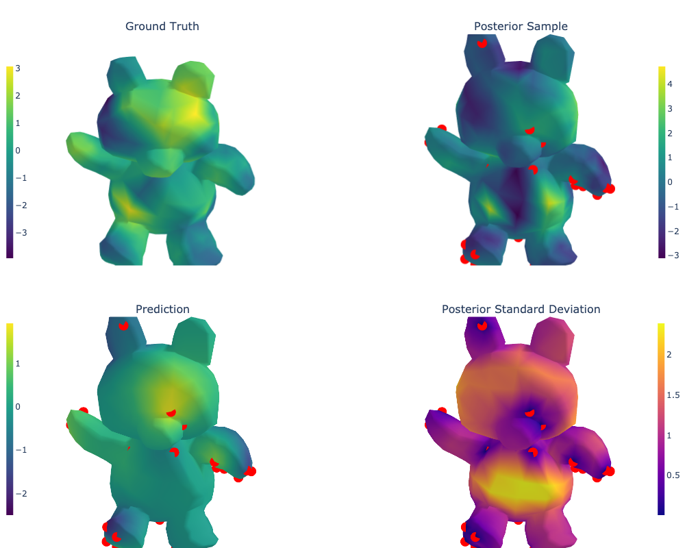
Data type cannot be displayed: application/vnd.plotly.v1+json

Citations

If you are using meshes and GeometricKernels, please consider citing

@article{mostowsky2024,
      title = {The GeometricKernels Package: Heat and Matérn Kernels for Geometric Learning on Manifolds, Meshes, and Graphs},
      author = {Peter Mostowsky and Vincent Dutordoir and Iskander Azangulov and Noémie Jaquier and Michael John Hutchinson and Aditya Ravuri and Leonel Rozo and Alexander Terenin and Viacheslav Borovitskiy},
      year = {2024},
      journal = {arXiv:2407.08086},
}

@inproceedings{borovitskiy2020,
    title={Matérn Gaussian processes on Riemannian manifolds},
    author={Viacheslav Borovitskiy and Alexander Terenin and Peter Mostowsky and Marc Peter Deisenroth},
    booktitle={Advances in Neural Information Processing Systems},
    year={2020}
}

@article{sharp2020,
    author={Nicholas Sharp and Keenan Crane},
    title={A Laplacian for Nonmanifold Triangle Meshes},
    journal={Computer Graphics Forum (SGP)},
    volume={39},
    number={5},
    year={2020}
}