# To run this in Google Colab, uncomment the following line
# !pip install geometric_kernels

# If you want to use a version of the library from a specific branch on GitHub,
# say, from the "devel" branch, uncomment the line below instead
# !pip install "git+https://github.com/geometric-kernels/GeometricKernels@devel"

Matérn and Heat Kernels on Hamming Graphs

This notebook shows how to define and evaluate kernels on q-ary Hamming graphs \(H(d,q)\) for modeling data encoded as categorical vectors with kernels that respect the geometry of the Hamming distance.

Note: If you need a kernel operating on categorical vectors where \(q\) varies between dimensions, you can useHammingGraph in conjunction with product kernels or product spaces.

Note: When \(q=2\), the Hamming graph \(H(d,2)\) reduces to the hypercube graph \(C^d = \{0, 1\}^d\) (see HypercubeGraph.ipynb).

At the very end of the notebook we also show how to construct approximate finite-dimensional feature maps for the kernels on the Hamming graph and how to use these to efficiently sample the Gaussian processes \(\mathrm{GP}(0, k)\).

Note: the points on the Hamming graph \(H(d,q)\) are integer vectors of size \(d\) where each component takes values in \(\{0, 1, ..., q-1\}\) (arrays of the suitable backend).

We use the numpy backend here.

Contents

• Basics

  • Defining a Space

  • Defining a Kernel

  • Evaluating Kernels on Random Inputs

  • Visualizing Kernels

• Feature Maps and Sampling

  • Defining a Feature Map

  • Efficient Sampling using Feature Maps

• Citation

Basics

# Import a backend, we use numpy in this example.
import numpy as np

# Import the geometric_kernels backend.
import geometric_kernels

# Note: if you are using a backend other than numpy,
# you _must_ uncomment one of the following lines
# import geometric_kernels.tensorflow
# import geometric_kernels.torch
# import geometric_kernels.jax

# Import a space and an appropriate kernel.
from geometric_kernels.spaces import HammingGraph
from geometric_kernels.kernels import MaternGeometricKernel

# We use networkx to visualize graphs
import networkx as nx

import matplotlib as mpl
import matplotlib.pyplot as plt

INFO (geometric_kernels): Numpy backend is enabled. To enable other backends, don't forget to `import geometric_kernels.*backend name*`.
INFO (geometric_kernels): We may be suppressing some logging of external libraries. To override the logging policy, call `logging.basicConfig`.

Defining a Space

First we create a GeometricKernels space that corresponds to the 4-dimensional ternary Hamming graph \(H(4,3)\), where each coordinate takes values in \(\{0, 1, 2\}\).

hamming_graph = HammingGraph(4,3)

Defining a Kernel

First, we create a generic Matérn kernel.

To initialize MaternGeometricKernel you just need to provide a Space object, in our case this is the hamming_graph we have just created above.

There is also an optional second parameter num which determines the order of approximation of the kernel (number of levels). There is a sensible default value for each of the spaces in the library, so change it only if you know what you are doing.

A brief account on theory behind the kernels on the Hamming graph space can be found on this documentation page.

kernel = MaternGeometricKernel(hamming_graph)

To support JAX, our classes do not keep variables you might want to differentiate over in their state. Instead, some methods take a params dictionary as input, returning its modified version.

The next line initializes the dictionary of kernel parameters params with some default values.

Note: our kernels do not provide the outputscale/variance parameter frequently used in Gaussian processes. However, it is usually trivial to add it by multiplying the kernel by an (optimizable) constant.

params = kernel.init_params()
print('params:', params)

params: {'nu': array([inf]), 'lengthscale': array([1.])}

To define two different kernels, Matern-3/2 and Matern-∞ (aka heat, RBF, squared exponential, diffusion), we need two different versions of params we define below.

Note: like in the Euclidean or the manifold case, and unlike the general graph case, the \(1/2, 3/2, 5/2\) are reasonable values of \(\nu\).

params["lengthscale"] = np.array([2.0])
params_32  = params.copy()
params_inf = params.copy()
del params
params_32["nu"]  = np.array([3/2])

params_inf["nu"] = np.array([np.inf])

Now two kernels are defined and we proceed to evaluating both on a set of random inputs.

Evaluating Kernels on Random Inputs

We start by sampling 3 (uniformly) random points on our graph. An explicit key parameter is needed to support JAX as one of the backends.

key = np.random.RandomState(1234)

key, xs = hamming_graph.random(key, 3)

print(xs, xs.dtype)

[[2 1 0 0]
 [0 1 1 1]
 [2 2 2 0]] int32

Now we evaluate the two kernel matrices.

kernel_mat_32  = kernel.K(params_32,  xs, xs)
kernel_mat_inf = kernel.K(params_inf, xs, xs)

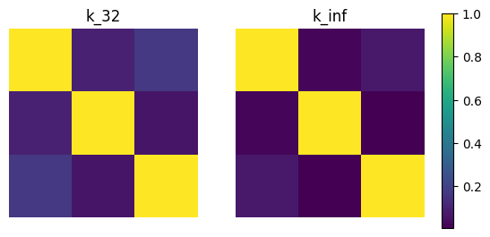
Finally, we visualize these matrices using imshow.

# find common range of values
minmin = np.min([np.min(kernel_mat_32), np.min(kernel_mat_inf)])
maxmax = np.max([np.max(kernel_mat_32), np.max(kernel_mat_inf)])

fig, (ax1, ax2) = plt.subplots(nrows=1, ncols=2)
cmap = plt.get_cmap('viridis')

ax1.imshow(kernel_mat_32, vmin=minmin, vmax=maxmax, cmap=cmap)
ax1.set_title('k_32')
ax1.set_axis_off()

ax2.imshow(kernel_mat_inf, vmin=minmin, vmax=maxmax, cmap=cmap)
ax2.set_title('k_inf')
ax2.set_axis_off()

# add space for color bar
fig.subplots_adjust(right=0.85)
cbar_ax = fig.add_axes([0.88, 0.25, 0.02, 0.5])

# add colorbar
sm = plt.cm.ScalarMappable(cmap=cmap,
                           norm=plt.Normalize(vmin=minmin, vmax=maxmax))
fig.colorbar(sm, cax=cbar_ax)

plt.show()

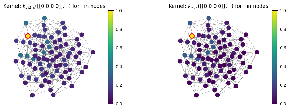
Visualizing Kernels

Here we visualize \(k_{\nu, \kappa}(\) base_point \(, x)\) for $x \in `$ ``other_points`. We define base_point and other_points in the next cell.

import itertools
base_point = np.array([0]*4)[None, :]  # choosing a fixed node for kernel visualization
other_points = np.array([list(i) for i in itertools.product([0, 1, 2], repeat=4)])

The next cell evaluates \(k_{\nu, \kappa}(\) base_point \(, x)\) for $x \in `$ ``other_points` for \(\nu\) either \(3/2\) or \(\infty\).

values_32  = kernel.K(params_32,  base_point,
                              other_points).flatten()
values_inf = kernel.K(params_inf, base_point,
                              other_points).flatten()

We prepare the networkx graph for visualizing the space

def hamming_graph_nx(d, q):
    """Create q-ary Hamming graph of dimension d."""
    G = nx.Graph()
    vertices = list(itertools.product(range(q), repeat=d))
    G.add_nodes_from(range(len(vertices)))

    for i, v1 in enumerate(vertices):
        for j, v2 in enumerate(vertices):
            if i < j and sum(a != b for a, b in zip(v1, v2)) == 1:
                G.add_edge(i, j)
    return G

nx_graph = hamming_graph_nx(4, 3)  # 81 vertices
pos = nx.spring_layout(nx_graph, seed=42)  # Auto-generate layout

Finally, we visualize the kernels

cmap = plt.get_cmap('viridis')

# Set the colorbar limits:
vmin = min(0.0, values_32.min(), values_inf.min())
vmax = max(1.0, values_32.max(), values_inf.max())


# Red outline for the base_point:
edgecolors = [(0, 0, 0, 0)]*nx_graph.number_of_nodes()
edgecolors[0] = (1, 0, 0, 1)

# Save graph layout so that graph appears the same in every plot
kwargs = {'pos': pos, 'node_size': 120, 'width': 0.2}


fig, (ax1, ax2) = plt.subplots(1, 2, figsize=(12.8, 4.))

# Plot kernel values 32
nx.draw(nx_graph, ax=ax1, cmap=cmap, node_color=values_32,
        vmin=vmin, vmax=vmax, edgecolors=edgecolors,
        linewidths=2.0, **kwargs)
sm = plt.cm.ScalarMappable(cmap=cmap,
                           norm=plt.Normalize(vmin=vmin, vmax=vmax))
cbar = plt.colorbar(sm, ax=ax1)
ax1.set_aspect(1)
ax1.set_title('Kernel: $k_{3/2, \kappa}($%s$, \cdot)$ for $\cdot$ in nodes' % str(base_point))

# Plot kernel values inf
nx.draw(nx_graph, ax=ax2, cmap=cmap, node_color=values_inf,
        vmin=vmin, vmax=vmax, edgecolors=edgecolors,
        linewidths=2.0, **kwargs)
sm = plt.cm.ScalarMappable(cmap=cmap,
                           norm=plt.Normalize(vmin=vmin, vmax=vmax))
cbar = plt.colorbar(sm, ax=ax2)
ax2.set_aspect(1)
ax2.set_title('Kernel: $k_{\infty, \kappa}($%s$, \cdot)$ for $\cdot$ in nodes' % str(base_point))


plt.show()

Feature Maps and Sampling

Here we show how to get an approximate finite-dimensional feature map for heat and Matérn kernels on the Hamming graph \(H(d,q)\), i.e. such \(\phi\) that

\[k(x, x') \approx \langle \phi(x), \phi(x') \rangle_{\mathbb{R}^M}.\]

This might be useful for speeding up computations. We showcase this below by showing how to efficiently sample the Gaussian process \(\mathrm{GP}(0, k)\).

For a brief theoretical introduction into feature maps, see this documentation page.

Defining a Feature Map

The simplest way to get an approximate finite-dimensional feature map is to use the default_feature_map function from geometric_kernels.kernels. It has an optional keyword argument num which determines the number of features, the \(M\) above. Below we rely on the default value of num.

from geometric_kernels.kernels import default_feature_map
from geometric_kernels.utils.utils import make_deterministic

feature_map = default_feature_map(kernel=kernel)
feature_map = make_deterministic(feature_map, key=key)

key, features = feature_map(xs, params_32, key=key)

The resulting feature_map is a function that takes the array of inputs and parameters of the kernel. There is also an optional parameter normalize that determines if \(\langle \phi(x), \phi(x) \rangle_{\mathbb{R}^M} \approx 1\) or not. For Hamming graphs, normalize follows the standard behavior of MaternKarhunenLoeveKernel, being True by default.

feature_map outputs a tuple. Its second element is \(\phi(x)\) evaluated at all inputs \(x\). Its first element contains the updated key for randomized feature maps. For default_feature_map on a HammingGraph space, the feature map is randomized (using RandomPhaseFeatureMapCompact), so the first element is the updated random state.

In the next cell, we evaluate the feature map at random points, using params_32 as kernel parameters. We check the basic property of the feature map: \(k(x, x') \approx \langle \phi(x), \phi(x') \rangle_{\mathbb{R}^M}\).

# xs are random points from above
_, embedding = feature_map(xs, params_32)

print('xs (shape = %s):\n%s' % (xs.shape, xs))
print('')
print('emedding (shape = %s):\n%s' % (embedding.shape, embedding))

kernel_mat_32  = kernel.K(params_32,  xs, xs)
kernel_mat_32_alt = np.matmul(embedding, embedding.T)

print('')
print('||k(xs, xs) - phi(xs) * phi(xs)^T|| =', np.linalg.norm(kernel_mat_32 - kernel_mat_32_alt))

xs (shape = (3, 4)):
[[2 1 0 0]
 [0 1 1 1]
 [2 2 2 0]]

emedding (shape = (3, 15000)):
[[ 0.00699769 -0.0137675   0.01248256 ...  0.01248256 -0.00563144
  -0.0081862 ]
 [ 0.00711193 -0.00349806 -0.00634317 ... -0.00634317 -0.00572338
   0.00415992]
 [ 0.00692829  0.00681548 -0.00617938 ... -0.00617938  0.00696949
  -0.00202625]]

||k(xs, xs) - phi(xs) * phi(xs)^T|| = 0.02531349719744118

Efficient Sampling using Feature Maps

GeometricKernels provides a simple tool to efficiently sample (without incurring cubic costs) the Gaussian process \(f \sim \mathrm{GP}(0, k)\), based on an approximate finite-dimensional feature map \(\phi\). The underlying machinery is briefly discussed in this documentation page.

The function sampler from geometric_kernels.sampling takes in a feature map and, optionally, the keyword argument s that specifies the number of samples to generate. It returns a function we name sample_paths.

sample_paths operates much like feature_map above: it takes in the points where to evaluate the samples and kernel parameters. Additionally, it takes in the keyword argument key that specifies randomness in the JAX style. sample_paths returns a tuple. Its first element is the updated key. Its second element is an array containing the value of samples evaluated at the input points.

from geometric_kernels.sampling import sampler

sample_paths = sampler(feature_map, s=2)

# introduce random state for reproducibility (optional)
# `key` is jax's terminology
key = np.random.RandomState(seed=1234)

# new random state is returned along with the samples
key, samples = sample_paths(xs, params_32, key=key)

print('Two samples evaluated at the xs are:')
print(samples)

Two samples evaluated at the xs are:
[[-130.9953739  -177.25877559]
 [  41.14356715  136.7170067 ]
 [  79.75263457 -217.72826631]]

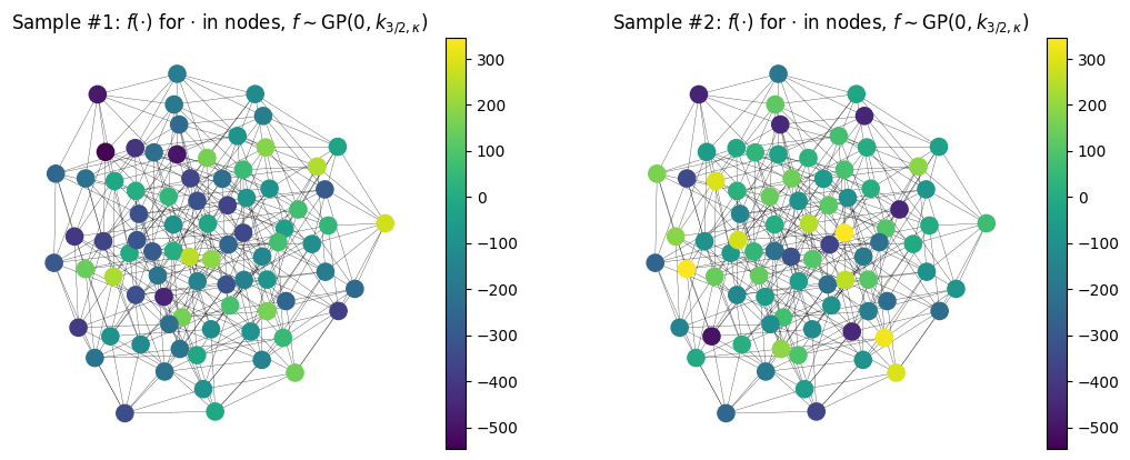
Visualizing Samples

Here we visualize samples as functions on a graph.

key = np.random.RandomState(seed=1234)
key, samples = sample_paths(other_points, params_32, key=key)

sample1 = samples[:, 0]
sample2 = samples[:, 1]

cmap = plt.get_cmap('viridis')

# Set the colorbar limits:
vmin = min(sample1.min(), sample2.min())
vmax = max(sample1.max(), sample2.max())

# Save graph layout so that graph appears the same in every plot
kwargs = {'pos': pos, 'node_size': 120, 'width': 0.2}

fig, (ax1, ax2) = plt.subplots(1, 2, figsize=(12.8, 4.8))

# Plot sample #1
nx.draw(nx_graph, ax=ax1, cmap=cmap, node_color=sample1,
        vmin=vmin, vmax=vmax, **kwargs)
sm = plt.cm.ScalarMappable(cmap=cmap,
                           norm=plt.Normalize(vmin=vmin, vmax=vmax))
cbar = plt.colorbar(sm, ax=ax1)
ax1.set_title('Sample #1: $f(\cdot)$ for $\cdot$ in nodes, $f \sim \mathrm{GP}(0, k_{3/2, \kappa})$')


# Plot sample #2
nx.draw(nx_graph, ax=ax2, cmap=cmap, node_color=sample2,
        vmin=vmin, vmax=vmax, **kwargs)
sm = plt.cm.ScalarMappable(cmap=cmap,
                           norm=plt.Normalize(vmin=vmin, vmax=vmax))
cbar = plt.colorbar(sm, ax=ax2)
ax2.set_title('Sample #2: $f(\cdot)$ for $\cdot$ in nodes, $f \sim \mathrm{GP}(0, k_{3/2, \kappa})$')

plt.show()

Citation

If you are using the HammingGraph space and GeometricKernels, please consider citing

@article{mostowsky2024,
      title = {The GeometricKernels Package: Heat and Matérn Kernels for Geometric Learning on Manifolds, Meshes, and Graphs},
      author = {Peter Mostowsky and Vincent Dutordoir and Iskander Azangulov and Noémie Jaquier and Michael John Hutchinson and Aditya Ravuri and Leonel Rozo and Alexander Terenin and Viacheslav Borovitskiy},
      year = {2024},
      journal = {arXiv:2407.08086},
}

@inproceedings{doumont2025,
    title = {Omnipresent Yet Overlooked: Heat Kernels in Combinatorial Bayesian Optimization},
    author = {Colin Doumont and Victor Picheny and Viacheslav Borovitskiy and Henry Moss},
    booktitle = {Advances in Neural Information Processing Systems},
    year = {2025},
}

@inproceedings{borovitskiy2023,
  title={Isotropic Gaussian Processes on Finite Spaces of Graphs},
  author={Borovitskiy, Viacheslav and Karimi, Mohammad Reza and Somnath, Vignesh Ram and Krause, Andreas},
  booktitle={International Conference on Artificial Intelligence and Statistics},
  year={2023},
}

@inproceedings{kondor2002,
    title={Diffusion Kernels on Graphs and Other Discrete Structures},
    author={Kondor, Risi Imre and Lafferty, John},
    booktitle={International Conference on Machine Learning},
    year={2002}
}